Analysis

Unless otherwise stated the GDP values are in the form log(GDP) for better visualization and interpretation

All data is shown up until 2019 in order to avoid COVID-19 affecting the data.

Introduction:

Originally we had data that was limited to U.S. travel counts to foreign countries. We decided we wanted to look at total passengers as a response variable. In order to determine why certain countries stood out, we implemented datasets containing figures such as population, GDP per capita, GDP growth, and overall GDP on a yearly basis from 1990-2019. Our main question became:

How does various countries’ GDP data affect the volume of US travel to that country?

Breadth of the DA:

We explore the effect of GDP, GDP per capita, and GDP growth on US travel. We also looked at some initial relationships between Total Passengers and variables contained in our first dataset such as Month and US Airport. We also attempted to observe a potential relationship between country population and incoming travel (Total Passengers). We did end up plotting a figure however it was relatively incoherent and not of much use. We found that our strongest support for our claims is within the GDP oriented variables such as GDP, GDP per capita, and GDP growth.

The plot below shows the relationship between total number of passengers departing from specific US Airports from 2010-2019. We were able to determine which airports had the highest traffic. This did not end up proving useful to our final conclusions although it was an initial step we took with limited data.

plane_data_clean %>%
group_by(US_Airport, Year) %>%
summarize(n = sum(Total)) %>%
arrange(Year, n) %>%
filter(n >= 1000000) %>%
filter(Year >= 2010, Year <= 2019) %>%
ggplot(aes(Year, n)) +
geom_line(aes(color = US_Airport)) +
labs(title = "Us Airport Traffic (Over 1 Million Flights) By Year: 2010-2019") +
xlab("Year") +
ylab("Number of Flights")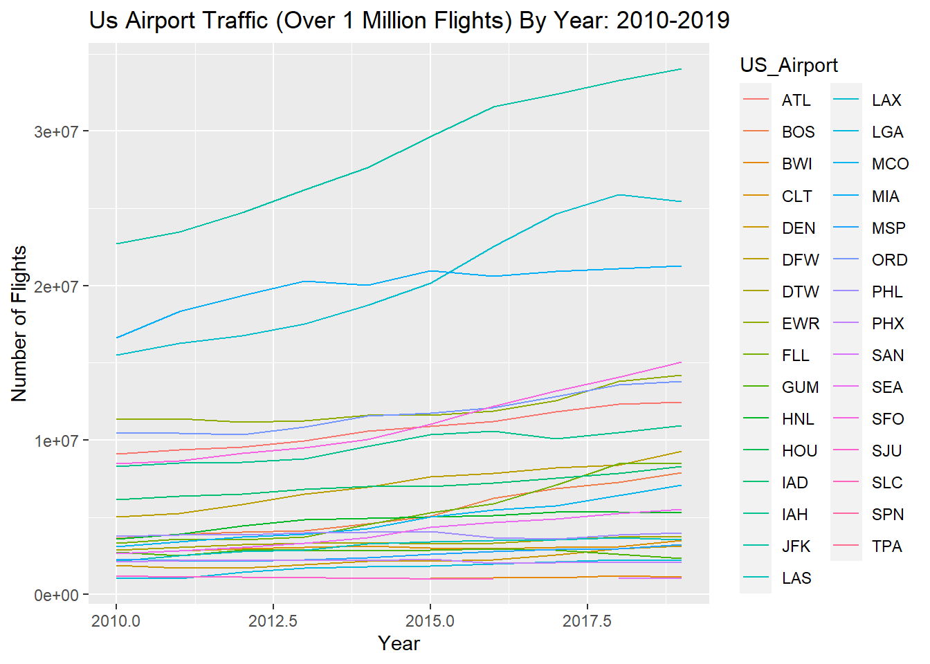

Another early exploration of ours featured attempting to determine which months had higher travel than others to see if there was any potential for analysis there. We determined that the holidays and the summers had higher travel, but again did not ultimately use these figures in our final conclusions.

plane_data_clean %>% group_by(Year, Month) %>% 
summarize(n = sum(Total)) %>% 
ggplot(aes(Year, n)) + geom_point(aes(color = as.factor(Month))) + labs(y = "Total Passengers")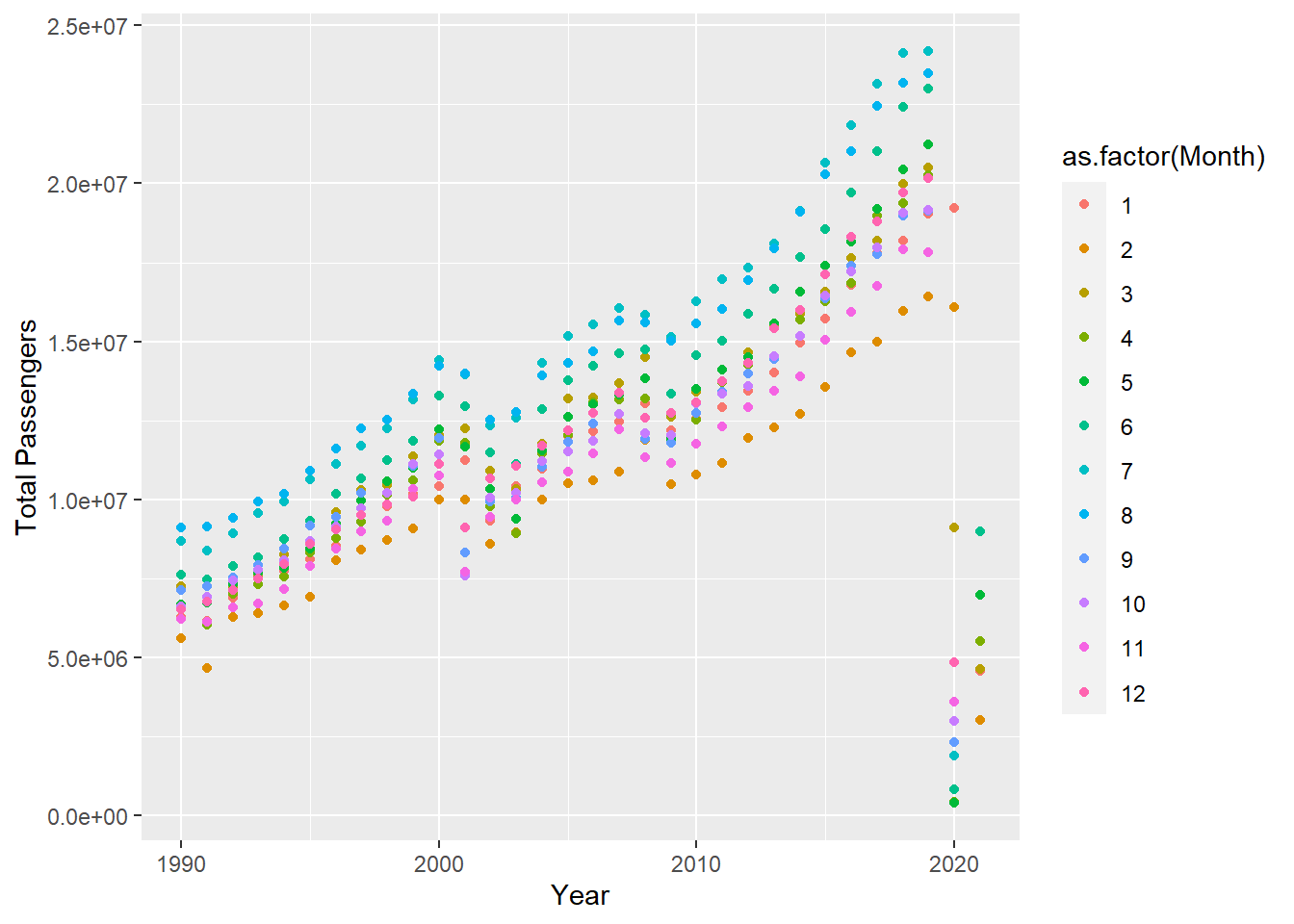

plane_data_clean %>% group_by(Month) %>%
summarize(n = sum(Total)) %>% filter(n >= 100000000) %>% 
ggplot(aes(as.factor(Month), n)) + geom_col() + labs(x = "Month", y = "Frequency")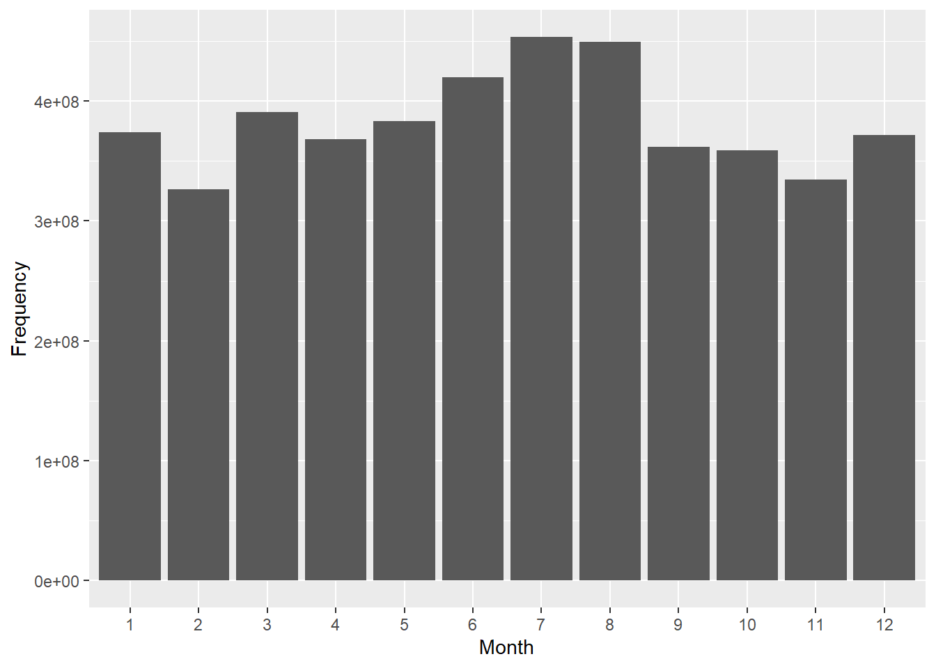

GDP per capita plotted against Total Passengers for high GDP countries, as we discovered that high GDP locations have a greater relationship between GDP increase and travel increase:

big_capita <- plane_data_join_GDP %>% filter(Year == 2019) %>%
group_by(Country) %>% transmute(FG_wac, GDPPerCapita) %>% arrange(desc(GDPPerCapita)) %>% unique() %>% head(20)
plane_data_join_GDP %>% 
filter(Year < 2020,FG_wac %in% big_capita$FG_wac) %>%
group_by(Year, Country) %>%
summarize(TotalPassengers = sum(Total), gdpPC = GDPPerCapita, Country) %>% unique() %>% 
ggplot(aes(gdpPC, TotalPassengers)) + geom_point(aes(color = Country)) + xlab("GDP Per Capita")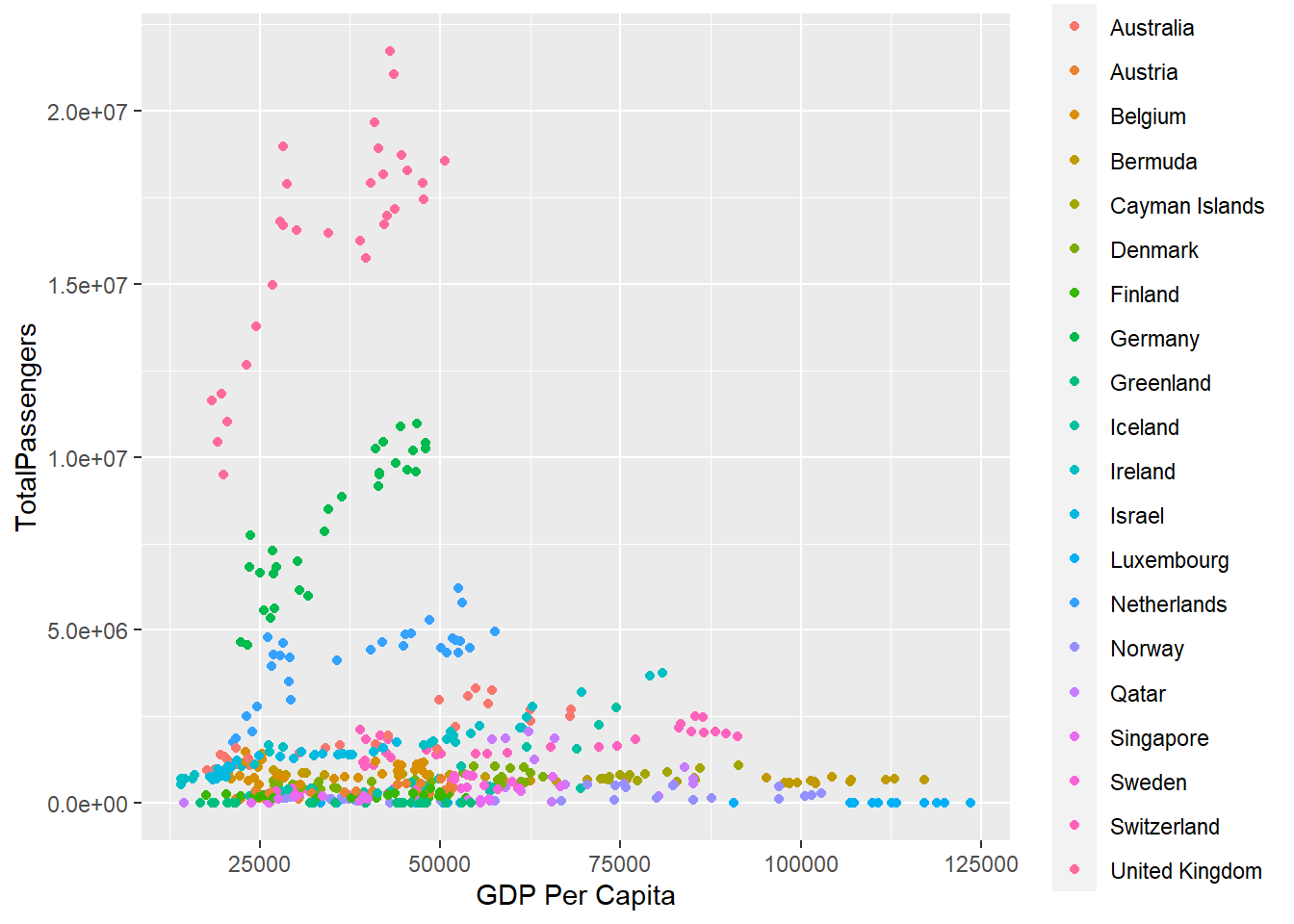

Total GDP vs. Total Passengers for the top 10 GDP Growth countries:

high_growth <- plane_data_join_GDP %>% filter(Year == 2019) %>% group_by(Country) %>% transmute(FG_wac, GDPGrowth) %>% arrange(desc(GDPGrowth)) %>% unique() %>% head(10)

plane_data_join_GDP %>% filter(Year < 2020,FG_wac %in% high_growth$FG_wac) %>% group_by(Year) %>%
summarize(TotalPassengers = sum(Total), gdp = log(GDP), Country) %>% unique() %>% ggplot(aes(gdp, TotalPassengers)) + geom_point(aes(color = Country)) + xlab("log(GDP)")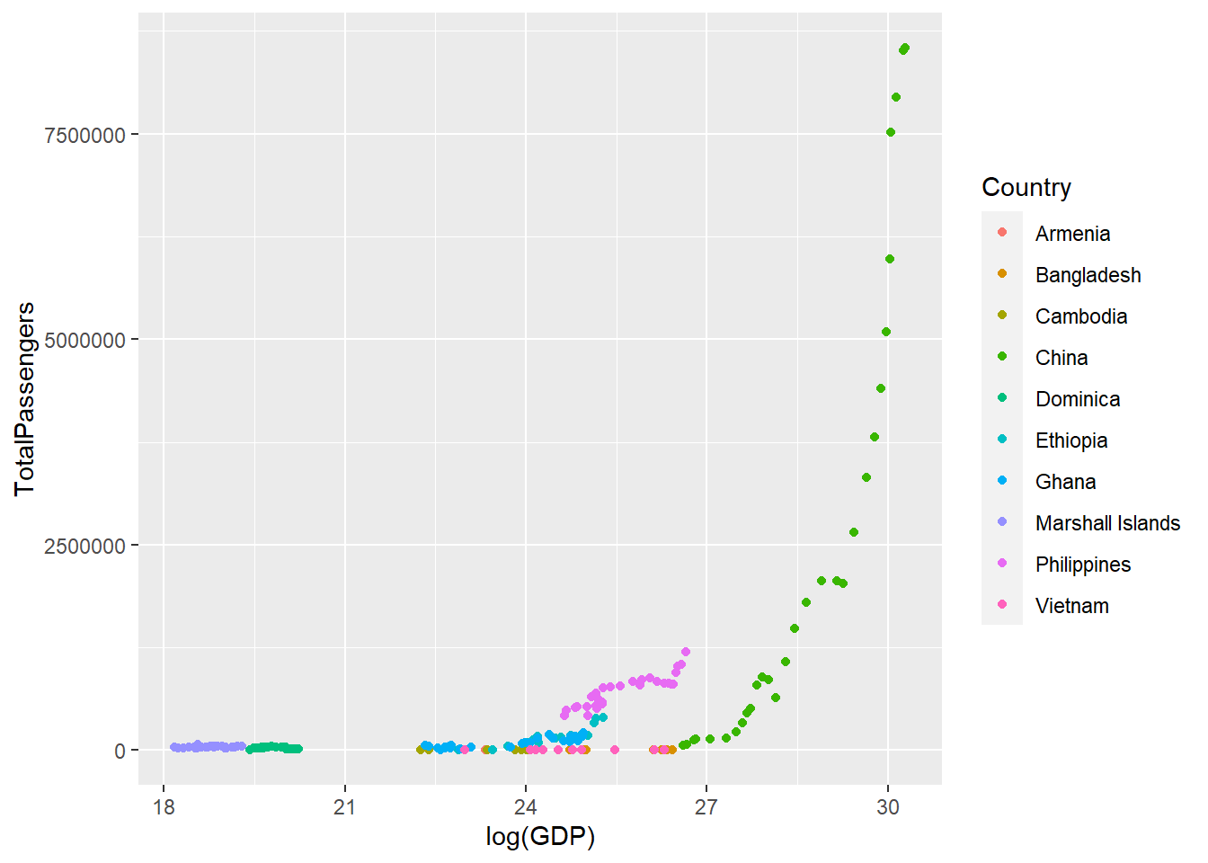

Depth of the DA

These countries were originally discovered to be the top GDP per capita countries, and we had previously determined that overall GDP influenced travel destinations, so now we looked in depth to see if already established high GDP per capita countries exhibited any relationship between GDP per capita and travel to that country.

GDP per capita for the standout selected countries (Ireland, Netherlands, Singapore):

irenetsin <- plane_data_join_GDP %>% filter(Year == 2019, FG_wac == "461" | FG_wac == "441" | FG_wac == "776") %>% 
group_by(Country) %>% transmute(FG_wac, GDPPerCapita) %>% arrange(desc(GDPPerCapita)) %>% unique()
plane_data_join_GDP %>% filter(Year < 2020,FG_wac %in% irenetsin$FG_wac) %>% group_by(Year, Country) %>% summarize(TotalPassengers = sum(Total), gdpPerCap = GDPPerCapita, Country) %>% unique() %>% 
ggplot(aes(gdpPerCap, TotalPassengers)) + geom_point(aes(color = Country)) + xlab("GDP per Capita")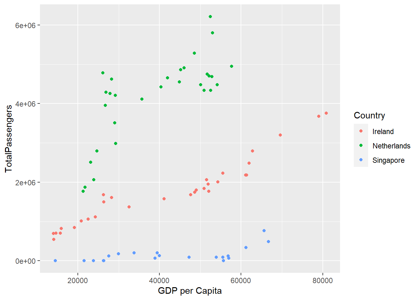

Displays an apparent positive linear relationship between all three of these countries, with Singapore’s being weaker but still visible, establishing evidence that high GDP per capita countries show increased travel as their GDP per capita increases as well.

Specific to the United Kingdom, one of the multiple countries we tested individually to determine if there was potential for further analysis, which we deemed there was. This plot does not feature log(GDP), just the raw GDP value.

plane_data_join_GDP %>% filter(Year < 2020, FG_wac == 493) %>% group_by(Year) %>% summarize(TotalPassengers = sum(Total), gdp = GDP) %>% unique() %>% ggplot(aes(gdp, TotalPassengers)) + geom_point()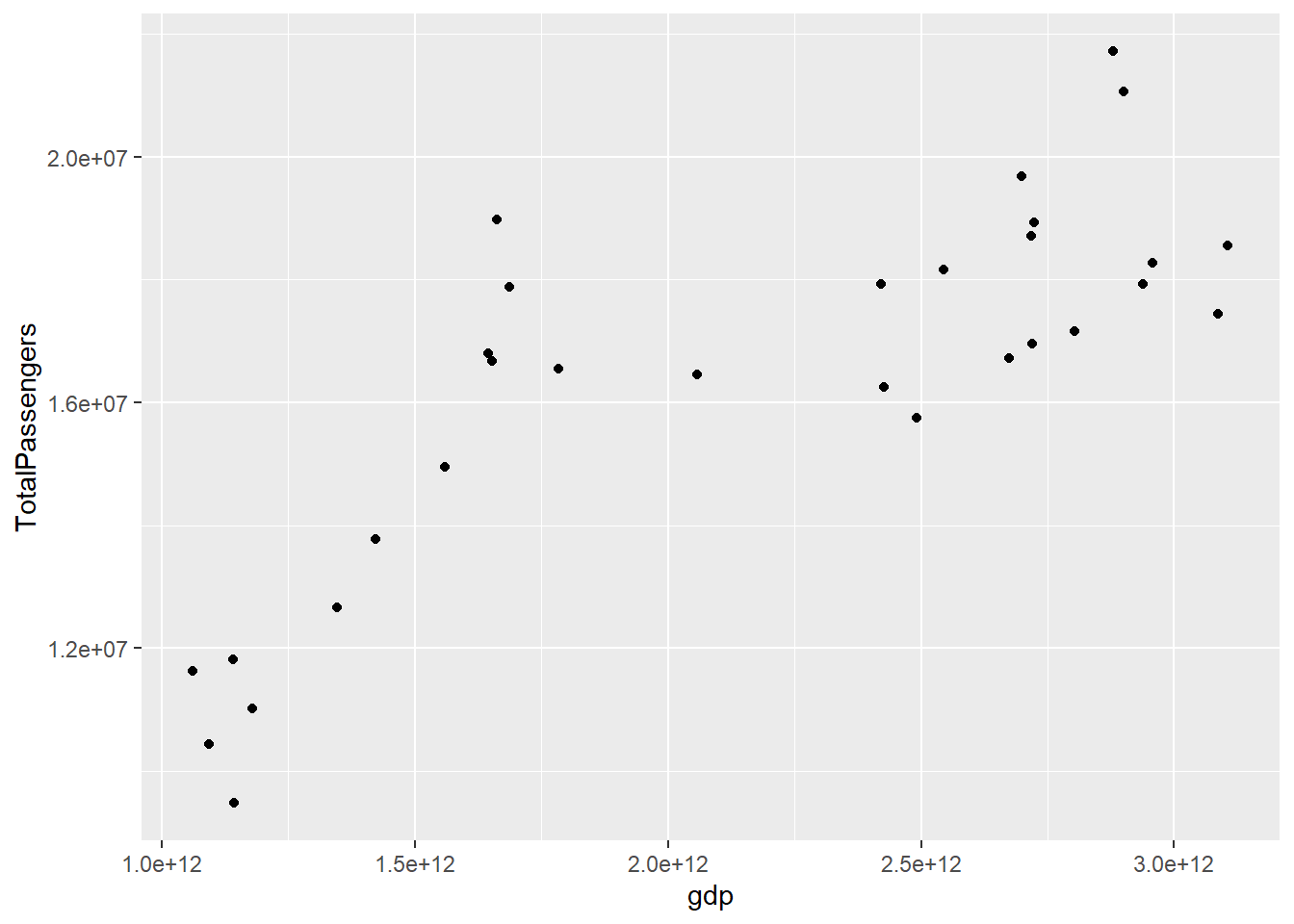

Modeling and Inference:

For our linear model we knew we wanted to focus on the relationship between GDP and Travel Volume. To begin with that we looked at Total Passengers as our dependent(response) variable, and the GDP value as our independent variable. We determined that through our earlier data exploration and analysis higher GDP growth rates resulted in higher travel traffic. Below are two models that examine that claim and highlight the facts we were able to find. These models do not feature log(GDP), because through model selection analysis we determined the most statistically significant values came from using purely GDP as a value.

countrydata <- plane_data_join_GDP %>% group_by(Country)
fitmodel <- lm(Total~GDP, data = countrydata)
summary(fitmodel)

## 
## Call:
## lm(formula = Total ~ GDP, data = countrydata)
## 
## Residuals:
##    Min     1Q Median     3Q    Max 
## -21564  -5693  -2356   2962 143070 
## 
## Coefficients:
##              Estimate Std. Error t value Pr(>|t|)    
## (Intercept) 5.966e+03  1.510e+01   395.2   <2e-16 ***
## GDP         1.060e-09  7.030e-12   150.7   <2e-16 ***
## ---
## Signif. codes:  0 '***' 0.001 '**' 0.01 '*' 0.05 '.' 0.1 ' ' 1
## 
## Residual standard error: 8640 on 484317 degrees of freedom
##   (214032 observations deleted due to missingness)
## Multiple R-squared:  0.0448, Adjusted R-squared:  0.0448 
## F-statistic: 2.272e+04 on 1 and 484317 DF,  p-value: < 2.2e-16

countrydata %>% 
ggplot(aes(GDP, Total)) + geom_point() + geom_abline(intercept = fitmodel$coefficients[1], slope = fitmodel$coefficients[2])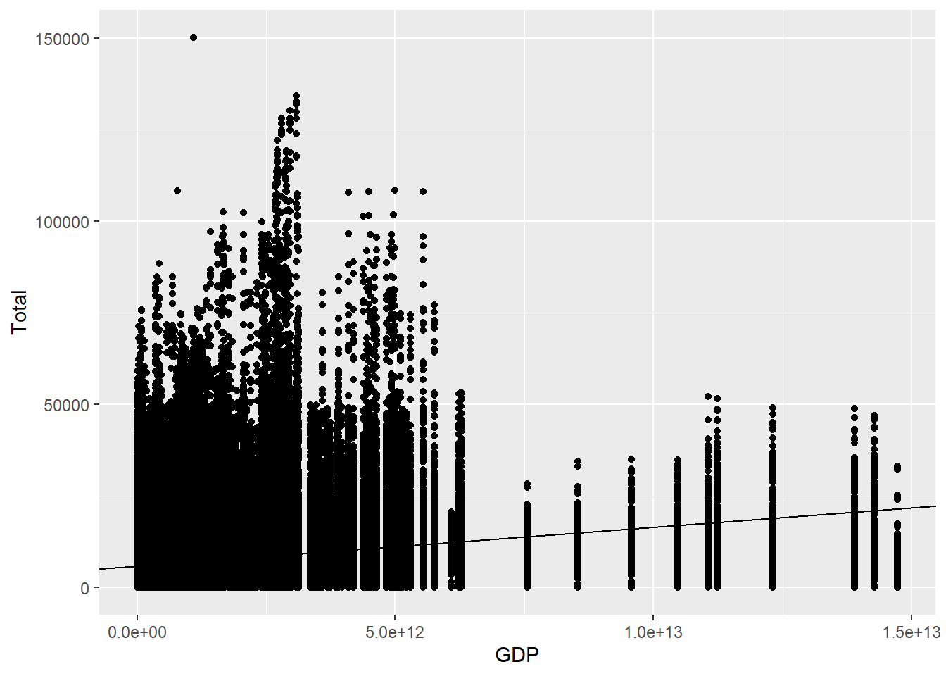

attach(countrydata)
cor.test(Total, GDP)

## 
##  Pearson's product-moment correlation
## 
## data:  Total and GDP
## t = 150.72, df = 484317, p-value < 2.2e-16
## alternative hypothesis: true correlation is not equal to 0
## 95 percent confidence interval:
##  0.2089784 0.2143587
## sample estimates:
##       cor 
## 0.2116701

This first model features every country’s Total Passenger count for a year plotted against the total GDP value for the same year and country. We were able to test the hypothesis that there was a significant relationship between Total and GDP within our entire cleaned dataset, and although the graph is semi-complex, there is a clear positive linear relationship. The summary statistics also display that the model has a p-value much lower than required to reject the null hypothesis, again furthering the claim that these two variables contain a statistically significant linear relationship. Finally, the large model has a correlation coefficient of .21 between Total and GDP, which although is not eye-poppingly large it is certainly significant enough to claim that the true correlation is not 0. This again reaffirms the relationship.

sgpdata <- plane_data_join_GDP %>% filter(FG_wac == 776)
fitsgp <- lm(Total~GDP, data = sgpdata)
summary(fitsgp)

## 
## Call:
## lm(formula = Total ~ GDP, data = sgpdata)
## 
## Residuals:
##      Min       1Q   Median       3Q      Max 
## -10224.7  -3857.5    367.4   3261.6  17988.6 
## 
## Coefficients:
##              Estimate Std. Error t value Pr(>|t|)    
## (Intercept) 1.322e+03  7.635e+02   1.731   0.0842 .  
## GDP         2.400e-08  2.700e-09   8.888   <2e-16 ***
## ---
## Signif. codes:  0 '***' 0.001 '**' 0.01 '*' 0.05 '.' 0.1 ' ' 1
## 
## Residual standard error: 5039 on 400 degrees of freedom
##   (12 observations deleted due to missingness)
## Multiple R-squared:  0.1649, Adjusted R-squared:  0.1628 
## F-statistic:    79 on 1 and 400 DF,  p-value: < 2.2e-16

sgpdata %>% 
ggplot(aes(GDP, Total)) + geom_point() + 
geom_abline(intercept = fitsgp$coefficients[1], slope = fitsgp$coefficients[2])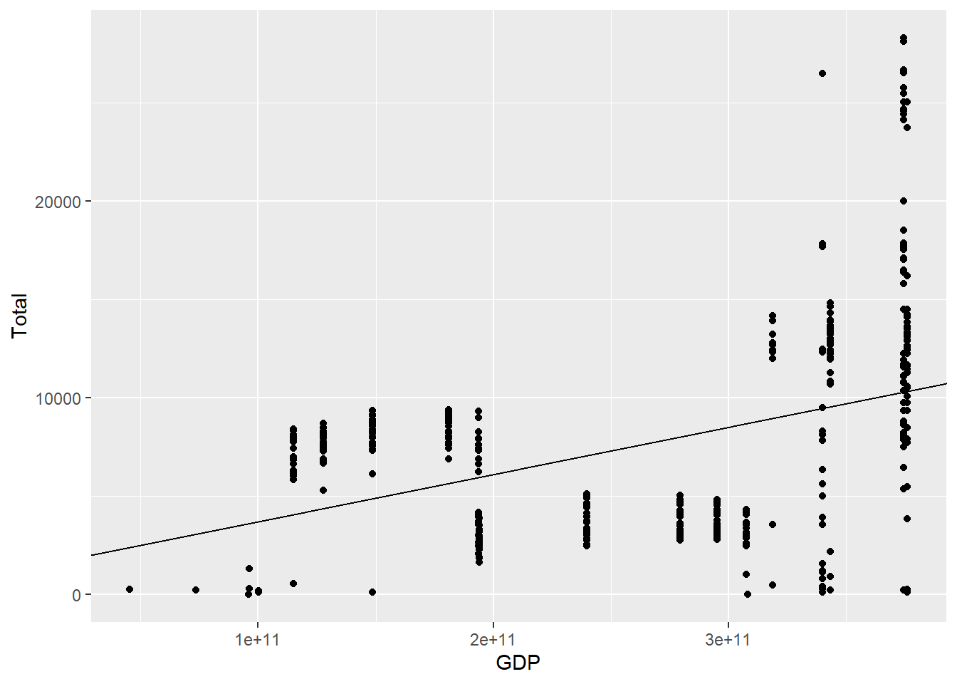

attach(sgpdata)
cor.test(Total, GDP)

## 
##  Pearson's product-moment correlation
## 
## data:  Total and GDP
## t = 8.8879, df = 400, p-value < 2.2e-16
## alternative hypothesis: true correlation is not equal to 0
## 95 percent confidence interval:
##  0.3210460 0.4846582
## sample estimates:
##       cor 
## 0.4061014

The second model we decided to implement was a further analysis on the relationship between Total Passengers and total GDP value for a specific country we determined had been experiencing high GDP growth during the years of our analysis. This model features only data from Singapore, again plotting raw GDP vs Total Passengers, with each year of data representing a point of data. This reduced model boasts a much larger F-value, a much lower p-value, and a correlation coefficient that is almost twice as high as the main model. This information combined with the obviously apparent positive linear relationship shown from the graph leads us to conclude that there is again a statistically significant relationship between GDP and Total Passengers in Singapore specifically. This conclusion led us to further pursue the fact that this relationship is more prevalent amongst high GDP growth countries. The R^2 value remains small for statistically significant models, however we have detected 16% of the total explanation on Total Passengers.

Flaws and Limitations:

The distance between a country and the US would affect the data. Some other data that would help would be this distance data. Another flaw is that many countries are used as international travel hubs, so even if many passengers go from the US to a certain country, there might not be many direct flights. Along with the missing variables that lead our model incomplete, we also were forced to assume certain relationships between GDP and Total Passengers were not collinearity between GDP and other predictors, whether those be used or hidden amongst other data. Our model did display that at least SOME of the relationship was due to the predictors chosen, however with other variables such as distance we could have potentially done even more analysis. Again, our data assumes that one of the main contributing factors to travel locations are their GDP values and figures and not some outside factors like hype, tourist attention, location, climate.